Using Variational AutoEncoders to Analyze Medical Images
Unsupervised learning is about inferring hidden structure from unlabelled data. There is no supervision in the form of labels, so the model has to figure out how to represent the data and find patterns in it. When we have large quantities of data, and none or few labels, the most effective technique is to use unsupervised methods to learn from data.
Why do we need it?
Deep learning methods which are popular today require large quantities of labelled data for training. Labelling is a very time consuming task and in case of medical images, requires significant time commitment from highly trained physicians with specialized skill-sets such as radiologists and pathologists. Lack of large datasets is by far the biggest challenge in applying Deep Learning techniques in the healthcare domain. One way, this can be mitigated is by using unsupervised methods to train on data without labels. These methods can learn patterns in the data which can then be clustered or used for supervised learning with small datasets.
The volume of medical data is growing at a rapid pace as was mentioned here. The data are usually from different modalities (as in case of MRI) or from different enviroments (machines, patients). Building a supervised model to handle all these situations means painstakingly labelling or annotating data from every various scenario. To tackle it, problem we need an approach which uses mix of supervised and unsupervised learning.
Unsupervised Methods in DL
The following methods are used for Unsupervised Learning using Deep Learning
- RBMs ( Restricted Boltzmann Machines )
- Sparse Coding
- AutoEncoders
- Generative Models (VAEs, GANs)
What are VAEs ( Variational AutoEncoders )
VAE stands for Variational AutoEncoders. It is a type of generative model which was introduced in the paper Auto Encoding Variational Bayes.
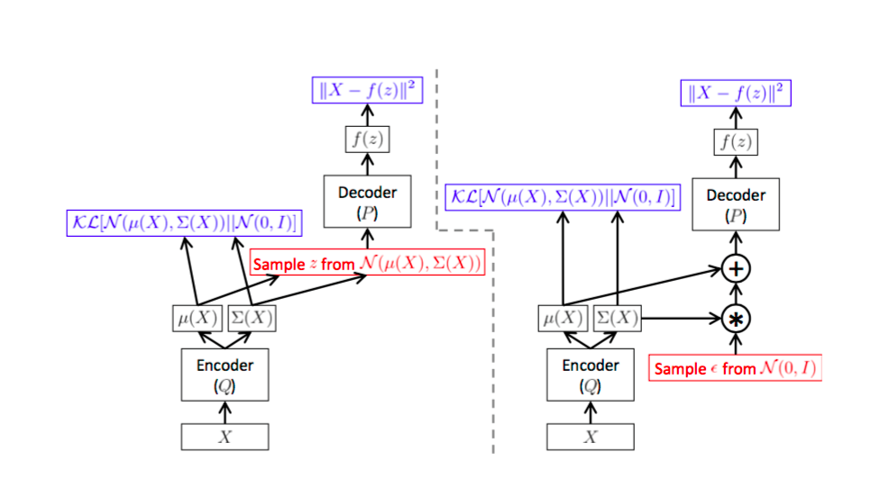
Architecture of the VAE. The left and right images represent the same VAE
The image illustrated above shows the architecture of a VAE. We see that the encoder part of the model i.e Q models the Q(z|X) (z is the latent representation and X the data). Q(z|X) is the part of the network that maps the data to the latent variables. The decoder part of the network is P which learns to regenerate the data using the latent variables as P(X|z). So far there is no difference between an autoencoder and a VAE. The difference is the constraint applied on z i.e the distribution of z is forced to be as close to Normal distribution as possible ( KL divergence term ).
Using a VAE we are able to fit a parametric distribution ( in this case gaussian ). This is what differentiates a VAE from a conventional autoencoder which relies only on the reconstruction cost. This means that during run time, when we want to draw samples from the network all we have to do is generate random samples from the Normal Distribution and feed it to the encoder P(X|z) which will generate the samples. This is shown in the figure below.
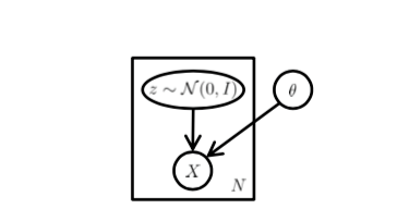
VAE as a graphical model and how to use it at runtime to generate samples
Objectives
Our goal here is to use the VAE to learn the hidden or latent representations of the data. Since this is an unsupervised approach we will only be using the data and not the labels. We will be using the VAE to map the data to the hidden or latent variables. We will then visualize these features to see if the model has learnt to differentiate between data from different labels.
Our first run will on the well known MNIST dataset. We will run the network on a dataset of two digits from the MNIST dataset and visualize the features the network has learnt. After this we will proceed to run the network on the ISLES 2015 dataset.
Running VAE on MNIST
Data
We will be using the Keras library for running our example. Keras also has an example implementation of VAE in their repository. We will be using this as our implementation. Here we will run an example of an autoencoder.
Data Preprocessing
MNIST dataset consists of 10 digits from 0-9. For our run we will choose only two digits (1 & 0).
Running the Network
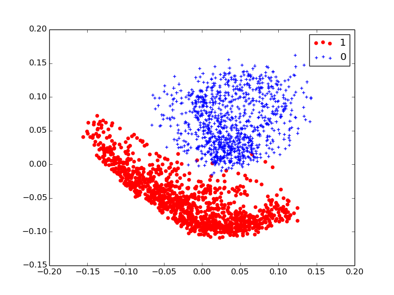
scatter plot of the latent representation
What we see here are two clusters one belonging to the digit 1 (red) and the other to the digit 0 (blue). The VAE has mapped the two different digits to different cluster in the latent variable space. The clusters are very well defined because the digits are structurally different.
Running on Medical Data
Data
For running VAE on a medical dataset we will use the Ischemic Lesion dataset. The dataset contains 28 scans of brains which have Ischemic lesion. It also contains the manually segmented masks of the lesion regions. There are four modalities of MRI image. (T1, T2, DWI, FLAIR).
Data Preprocessing
We will only be using the DWI modality. This is because Ischemic Lesions are visible in the DWI channel. For the preprocessing step we will be using SimpleITK to normalize the images. We also ensure the pixel values are scaled down to (0,1) range.
The next step is to extract 28x28 non overlapping patches from the 3D images. We will be reusing the same type of network as we used for the MNIST example. While extracting 28x28 non overlapping patches we also keep track of which patches have lesion regions and which are healthy patches.
Running the Network
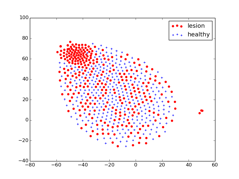
TSNE plot of the latent representation. blue colored dots are lesion patches red colored dots are healthy patches
The image illustrated above is the TSNE plot of the latent representations (dimension of z is 5) of the data.We can clearly see the data clustered into two groups. The center blue cluster which is free of any red dots is the lesion patches. Outer regions consisnt of a mixture red and blue dots. This can be explained by the fact that many lesion patches will have only a few pixels of lesion in them making it difficult to differentiate between them.
Next
In the next part we will explore how to improve clustering.