Visualizing Deep Learning Networks - Part I
At Qure, we’re building deep learning systems which help diagnose abnormalities from medical images. Most of the deep learning models are classification models which predict a probability of abnormality from a scan. However, just the probability score of the abnormality doesn’t amount much to a radiologist if it’s not accompanied by a visual interpretation of the model’s decision.
Interpretability of deep learning models is very much an active area of research and it becomes an even more crucial part of solutions in medical imaging.
The prevalent visualization methods can be broadly classified into 2 categories:
- Perturbation based visualizations
- Backpropagation based visualizations
In this post, I’ll be giving a brief overview of the different perturbation based techniques for deep learning based classification models and their drawbacks. We would be following up with backpropagation based visualisations methods in the next part of the series.

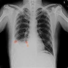
Chest X-ray with pleural effusion.
For context, we would be considering chest X-ray (image above) of a patient diagnosed with pleural effusion. A pleural effusion is a clinical condition when pulmonary fluids have accumulated in the pulmonary fields. A visual cue for such an accumulation is the blunting of costophrenic (CP) angle as shown in the X-ray shown here. As is evident, the left CP angle (the one in the right of the image) is sharp whereas the right CP angle is blunted indicating symptoms of pleural effusion.
We would be considering this X-ray and one of our models trained for detecting pleural effusion for demonstration purposes. For this patient, our pleural effusion algorithms predict a possible pleural effusion with 97.62% probability.
Perturbation visualizations
Methods
This broad category of perturbation techniques involve perturbing the pixel intensity of input image with minimum noise and observing the change of prediction probability. The underlying principle being that the pixels which contribute maximally to the prediction, once altered, would drop the probability by the maximum amount. Let’s have an overview glance at some of these methods - I’ve linked the paper for your further reading.
Occlusion
In the paper Visualizing and Understanding Convolutional Networks, published in 2013, Zeiler et al used deconvolutional layers - earliest applications of deconvolutional layers - to visualize the activity maps for each layer for different inputs. This helped the authors in understanding object categories responsible for activation in a given feature map. The authors also explored the technique of occluding patches of the network and monitoring the prediction and activations of feature map in the last layer that was maximally activated for unoccluded images.
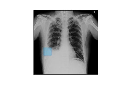
Here’s a small demo of how perturbation by occlusion works for the demo X-ray.
The leftmost image is the original X-ray image, the middle one is the perturbed image as the black occluding patch moves across the image, the rightmost image is the plot of the probability of pleural effusion as different parts of the X-ray gets occluded.
As is evident from above, the probability of pleural effusion drops as soon as the right CP angle and accumulated fluid region of the X-ray is occluded to the network, the probability of the pleural effusion drops suddenly. This signals the presence of blunt CP angle along with the fluid accumulation as the attributing factor pleural effusion diagnosis for the patient.
The same idea was explored in depth in the Samek et al in the 2015 paper Evaluating the visualization of what a Deep Neural Network has learned where authors suggests that we select the top k pixels by attribution and randomly vary their intensities and then measure the drop in score. If the attribution method is good, then the drop in score should be large.
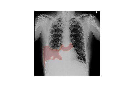
Here’s how the heatmap generated via occlusion would look like
Heatmap generated by occlusion
Super-pixel perturbation
But there’s a slight problem with occluding patches in a systematic way in regular grids. Often the object that is to be identified gets occluded in parts resulting in inappropriate decision by the network.
These sort of situations were better tackled in the LIME paper that came out in 2016. LIME isn’t specifically about computer vision but as such for any classifier. I’ll explain how LIME works for vision techniques explicitly and leave the rest for your reading. Instead of occluding systematic patches at regular intervals, input image is divided into component superpixels. A superpixel is a grouping of adjacent pixels which are of similar intensities. Thus grouping by superpixels ensures an object, composed of of similar pixel intensities, is a single superpixel component in itself.
The algorithm for generating heatmap goes as follows
- Image is segmented into component superpixels
- Generate k samples by
- Randomly activating some of the component superpixels. Activating a superpixel implies retaining intensities in superpixel to original values
- For non-activated superpixels, replace each superpixel component with corresponding average intensity of all pixels in the superpixel
- Generate predictions for each of the samples
- Fit a simple regression using k points - features being activation (or non-activation) of superpixels (1 if a superpixel is activated in the sample, 0 otherwise) in a sample and corresponding prediction for the sample as target.
- Use the weights of each superpixel feature to generate final heatmap
Here’s a demo of how superpixel based perturbation (LIME model) works for the demo X-ray.
The leftmost image is the original X-ray, the center plot shows perturbed images (out of the k samples) with different superpixels being activated. The rightmost one is scatter plot of probability for pleural effusion vs no. of activated superpixels in sample.
Here’s how heatmap generated through superpixel based perturbation would look like
Heatmap generated by LIME Model using superpixel based perturbation
However, these techniques still have some downfalls. Occlusion of patches, systematic or superpixelwise can drastically affect the prediction of networks. For e.g.- at Qure we had trained nets for diagnosing abnormalities from Chest X Rays. Chest X Rays are generally grayscale images and abnormalities could include any thing like unlikely opacity at any place, or enlarged heart etc. Now with partial occlusion, resultant images would be abnormal images since a sudden black patch in the middle of X Ray is very well likely to be an abnormal case.
Integrated Gradients
Instead of discretely occluding, another way to perturb images over a continuous spectrum were explored in a recent paper Axiomatic Attribution for Deep Networks. These models is in a way hybrid of gradient based methods & perturbation based methods. Here, the images are perturbed over a continuos domain from baseline image (all zeroes) to the current image, and sensitivity of each pixel with respect to prediction is integrated over the spectrum to give approximate attribution score for each pixel.
The algorithm for generating heatmap for input image X with pixel intensities xij goes as follows
- Generate k samples by varying pixel intensities linearly from 0 to xij
- Generate sensitivity of each pixel ∂a(x)/∂xij for each samples
- Integrate the sensitivity of each pixel over k samples to obtain final heatmap
Here’s a demo of how integrated gradients model works for the demo X-ray.
The leftmost image is the original X-ray, the center plot shows images as intensities are varied linearly from 0 to original intensity. The rightmost plot displays the sensitivity maps for each of the perturbed images as the intensities vary.
As you can observe, the sensitivity map is random and dispersed across the entire image in the begining when samples are closer to baseline image. As the image becomes closer to the original image, the sensitivity maps become more localised indicating the strong attribution of CP angle and fluid-filled areas to final prediction.
Here’s how heatmap generated through IntegratedGradients based perturbation would look like
Heatmap generated by Integrated Gradients
Finally, we discuss briefly about the most recent works of Fong et al in the paper Interpretable Explanations of Black Boxes by Meaningful Perturbation. In this paper the authors try and refine the heatmap mask of images, generated by sensitivity maps or otherwise, to fins the minimal mask to describe saliency. The goal of such a technique is to find the smallest subset of the image that preserves the prediction score. The method perturbs the sensitivity heatmap and monitors the probability drop to refine the heatmap to minimum pixels that can preserve the prediction score.
Discussions
While most of these methods do a decently good job of producing relevant heatmaps. There are couple of drawbacks to perturbation based heatmaps which make them unsuitable for real time deployment.
Computationally Expensive : Most of these models are run multiple feed-forwards for computing a single heatmap for a given input image. This makes the algorithms slow and expensive and thereby unfit for deployment.
Unstable to surprise artifacts : As discussed above, a sudden perturbation in the form of a blurred or an occluded patch is something the net is not familiar with from it’s training set. The predictions for such a perturbed image becomes skewed a lot making the inferences from such a technique uninterpretable. A screening model trained for looking at abnormalities from normal X Rays, would predict abnormality whenever such a perturbed image is presented to it.
The drawbacks around unstable artifacts are mostly overcome by Integrated Gradients and resulting in much more stable heatmaps.
The backpropagation based methods are much cheaper computationally than perturbation based methods and would be discussed in the next part of the blog post.